Uncertainty is not the enemy of truth it is the measure of our respect for it. A number without an error bar is not scientific precision. It is the oldest, most reliable warning sign of greenwashing.
Every carbon project eventually faces a version of the same demand: give us a number. How many tonnes are sequestered in this forest? How much did emissions fall this monitoring period? What is the baseline against which we should measure the project's impact? The market wants a single, clean integer the kind that fits neatly on a certificate, flows effortlessly into an ESG disclosure, and satisfies an auditor's checklist without generating further questions. That number is, in a rigorous scientific sense, a fiction.
This is not a flaw in the underlying science. It is an honest, unavoidable property of measuring complex biological systems at landscape scale. A forest is not a warehouse of identically stacked, uniformly sized carbon boxes. Trees grow at rates shaped by microclimate, soil chemistry, and species genetics. They die without notice. They store carbon across root systems, litter layers, and organic soil horizons that no satellite sensor can directly observe. Every carbon stock estimate is, when properly understood, a probability distribution a range of plausible values within which the true quantity sits, at a confidence level determined entirely by the rigour of the monitoring system that produced it.
The carbon market's convention of publishing single-point estimates stripped of confidence intervals is not a technical inevitability. It is a cultural choice one that protects transactional simplicity at a direct cost to scientific integrity. Buyers cannot price risk they cannot see. Regulators cannot mandate quality they cannot measure. Credits will increasingly be priced not just on their stated quantity but on the statistical confidence with which that quantity was established. Markets, developers, and institutional buyers that build for this transition now will hold a durable structural advantage over those still operating in the comfortable fiction of exact numbers.
The Four Sources of the Error Bar
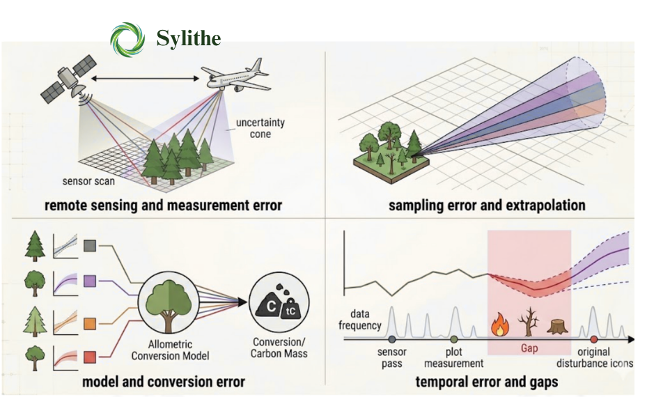
Uncertainty in carbon monitoring is not a single, undifferentiated cloud of imprecision. It originates from four structurally distinct phases of the MRV pipeline, each generating its own error component through different mechanisms, at different points in the workflow, and requiring different targeted interventions to reduce. Driving down the total error bar demands mapping precisely where each component originates.
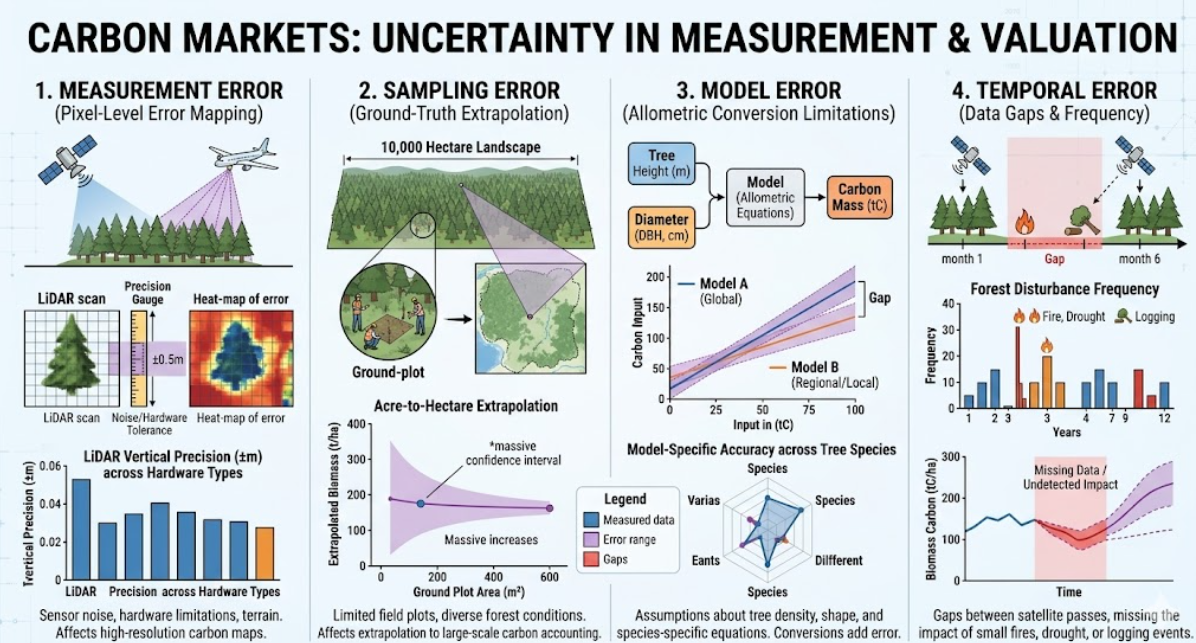
1. Measurement Error
Measurement error originates in the physics of the instruments themselves. Every sensor a satellite multispectral imager, an airborne LiDAR scanner, a handheld field dendrometer has fundamental hardware precision limits and introduces systematic and random noise into every observation. This is not a manufacturing defect. It is an intrinsic property of all physical measurement systems operating in the real world.
LiDAR systems measure canopy height by timing the return of laser pulses from vegetation and ground surfaces. Vertical precision for airborne LiDAR is typically 10–15 cm under open, optimal conditions but degrades significantly in dense tropical canopy, where overlapping returns from multiple canopy layers require complex waveform decomposition, in steep terrain, where scan-angle geometry introduces positional distortions, and in humid environments, where atmospheric water vapour affects pulse propagation timing. Any project claiming sub-5-centimetre LiDAR precision across a heterogeneous tropical forest is making a hardware claim that demands immediate scrutiny.
Satellite-based sensors carry their own distinct error profiles. SAR which enables the cloud-penetrating monitoring critical to tropical projects generates speckle noise as a fundamental property of coherent radar imaging. Multi-look filtering reduces this noise but introduces spatial averaging that blurs fine-scale biomass heterogeneity. Multispectral optical sensors face spectral saturation in dense, high-biomass canopy: the vegetation indices that correlate with biomass plateau above a density threshold, producing systematic underestimates of carbon stock in precisely the stands where carbon density is greatest. Characterising these limitations is not optional refinement it is the foundation on which every downstream uncertainty estimate depends.
2. Sampling Error
Sampling error enters through the necessary process of extrapolating from a finite set of measured ground-truth plots to the full project landscape. No project measures every tree across 50,000 hectares of forest. Instead, a statistically designed sample of field plots typically 0.1 to 0.5 hectares each is established, measured, and used to calibrate the relationship between remotely sensed signals and actual carbon stock. The precision of this extrapolation is determined by the sampling design, not by the sensors.
Three variables govern the size of sampling error: plot count (more plots yield lower uncertainty, with diminishing returns as sample size grows), spatial distribution (stratified random sampling across the full range of forest conditions is statistically superior to convenience sampling concentrated along accessible corridors), and the intrinsic variability of the forest type being sampled (a heterogeneous mixed-species tropical forest requires substantially more plots to characterise than a structurally uniform plantation). These three factors interact: a large number of plots clustered in accessible valley bottoms produces greater sampling uncertainty than a smaller, well-designed stratified sample spanning the full range of forest conditions.
Sampling error is fully quantifiable using standard statistical methods it is not inherently unknowable. But honest quantification requires a sampling design that is fit for purpose from the outset. Projects that deploy field plots in accessible, visually representative areas and extrapolate to the full landscape without statistically accounting for selection bias are understating their actual sampling uncertainty by a material margin. The stated confidence interval is narrower than the true knowledge the data supports a form of precision that exists on paper but not in the forest.
3. Model Error
Even where measurement and sampling are conducted with full statistical rigour, a third uncertainty source enters through the allometric models used to convert observable tree dimensions height, diameter at breast height, crown diameter into estimates of above-ground biomass and, subsequently, into carbon mass. These models are not physical laws. They are empirical regression relationships estimated from datasets of felled and weighed trees, and they carry their own irreducible uncertainty.
Pan-tropical allometric equations the most widely used family of models in tropical forest carbon projects were calibrated on tree datasets aggregated across forest types spanning multiple continents. Applied to a specific forest community in the Western Ghats, the Andaman Islands, or the forests of Assam, they are approximations built on training data that may share few species in common with the target ecosystem. The model's residual error term, compounded by the natural variability in wood density across species, age classes, and site conditions, propagates through every biomass and carbon estimate in the project. It cannot be subtracted out by better sensors or more field plots.
In temperate forests with long research histories and region-specific allometric equations, model uncertainty may contribute 10–15% to the total above-ground biomass estimate. In less-studied tropical forest types where pan-tropical equations are the only available option, that contribution can reach 20–30%. Projects that do not disclose which specific allometric equations they apply, or that use pan-tropical models for geographically specific forest types without acknowledging the resulting uncertainty penalty, are presenting buyers with a model error that has been made invisible by omission.
4. Temporal Error
The fourth source of uncertainty operates across a dimension that sensor resolution and plot count cannot address: time. Carbon monitoring is not a single snapshot it is a time series. Carbon stocks shift continuously as trees grow, are killed by competition, drought, or disease, and as forest structure is reshaped by storms, fire, and anthropogenic disturbance. Temporal error accumulates during the gaps between observations windows during which real-world changes in carbon stock are invisible to the monitoring system.
Monitoring cadence determines temporal exposure. A system with reliable monthly clear-sky optical coverage faces shorter observation gaps than one dependent on quarterly scene acquisitions. In cloud-prone tropical regions which contain a disproportionate share of the world's high-carbon-density forests optical satellite imagery may be entirely unavailable for weeks or months during monsoon seasons. These are temporal blind spots. If a disturbance event a localised fire, an illegal clearing incursion, a windthrow occurs within one of these gaps, the carbon loss is not detected until the next clear acquisition. Credits issued during the interval between the event and its detection can materially overstate the project's actual carbon stock.
SAR satellites resolve the cloud-penetration problem imaging continuously through monsoon cover but introduce their own biomass estimation model error, which increases with above-ground biomass density due to signal saturation in high-canopy forests. This is the fundamental sensor diversity problem: no single sensor type eliminates all four uncertainty components simultaneously. Minimising temporal error in high-value tropical carbon monitoring requires a multi-sensor architecture combining the all-weather availability of SAR, the spectral richness of optical imagery, and the structural precision of periodic LiDAR to maintain continuous, high-confidence coverage across all atmospheric conditions.
Why Human Beings Hate Error Bars
One reason uncertainty remains poorly communicated in carbon markets is psychological rather than technical. Human beings naturally prefer certainty. Investors prefer deterministic forecasts. Executives prefer clean dashboards. Buyers prefer simple numbers that can be communicated internally without lengthy statistical explanations. A number accompanied by an error bar requires a more complex conversation than a number presented alone. Complexity reduces transaction velocity. Uncertainty, in the short term, is commercially inconvenient.
Unfortunately, nature does not operate according to these preferences.
Every scientific discipline that measures complex systems eventually confronts this same tension. Meteorologists provide probability-based forecasts. Epidemiologists publish confidence intervals. Financial institutions evaluate risk distributions rather than guaranteed outcomes. Climate scientists report ranges rather than single values. In each case, the discipline eventually reached the conclusion that honest communication of uncertainty, even when it complicates the message, produces more reliable long-term outcomes than false precision.
Carbon markets are following the same path, but the journey has been slower than in other fields. The voluntary carbon market emerged primarily as a commercial ecosystem driven by transaction volume and credit issuance. In that environment, technical complexity was often subordinated to market accessibility. The simpler the number, the easier the sale. This was a reasonable early-stage design choice. But as markets mature and institutional capital enters, the standards of evidence naturally rise.
The presence of uncertainty does not weaken a carbon estimate. It strengthens it. A carbon stock estimate accompanied by a transparent confidence interval is more trustworthy than a larger estimate presented without uncertainty disclosure, because it demonstrates that the measurement system is sophisticated enough to know what it does not know. Counterintuitively, a well-characterised error bar signals methodological maturity rather than methodological weakness.
In many cases, the most dangerous number is not one with a large error bar. It is a number with no error bar at all. The absence of uncertainty reporting does not mean uncertainty is absent. It means it has been suppressed, ignored, or never quantified. Buyers who accept undisclosed uncertainty are not avoiding risk. They are accepting it invisibly.
The future carbon market will increasingly reward projects that disclose uncertainty honestly rather than those that attempt to conceal it behind false precision. As verification standards tighten and institutional buyers develop more sophisticated due diligence frameworks, the capacity to quantify and communicate uncertainty transparently will become a quality signal rather than a liability.
Why Forests Are Harder To Measure Than Factories
A manufacturing facility operates within a controlled environment. Inputs are metered. Outputs are measured. Production systems behave according to engineering specifications that change relatively slowly and predictably. The uncertainty in an industrial emissions estimate arises primarily from measurement precision and reporting quality, both of which can be managed through standardised instrumentation and audit procedures. Industrial carbon accounting, while imperfect, benefits from the relative tractability of controlled systems.
Forests do not.
A forest is a living adaptive system influenced simultaneously by climate variability, soil geochemistry, species interactions, mycorrhizal networks, disease pressure, herbivory, disturbance events, fire regimes, and human activity. Carbon stocks are not stored in uniform containers. They are distributed across millions of individual biological entities trees, shrubs, understorey vegetation, roots, litter, deadwood, and soil organic matter each of which changes continuously over time in ways that are influenced by dozens of interacting environmental variables.
This biological complexity creates monitoring challenges that have no industrial equivalent. Tree growth rates differ not only between species but between individuals of the same species growing in adjacent plots under subtly different microclimate conditions. Carbon density varies dramatically between forest patches separated by only a few hundred metres of altitude, aspect, or soil depth. Remote sensing signals change seasonally as leaf area index fluctuates, phenological cycles advance, and atmospheric water vapour affects radiometric quality. Disturbances can alter biomass suddenly and catastrophically, without warning and without detection between monitoring intervals.
These realities make forest carbon accounting fundamentally different from industrial emissions accounting. Measuring a forest is closer to characterising a dynamic ecosystem than auditing a balance sheet. The question is not simply whether trees exist. The question is how much carbon those trees contain, how that carbon is distributed spatially, how it is changing temporally, and how confident we can be in each component of that assessment.
The challenge is not obtaining a number. Carbon monitoring systems can always produce a number. The challenge is understanding how confident we should be in that number and whether that confidence has been honestly characterised or quietly inflated.
Forest carbon projects that reach institutional-grade monitoring quality are not merely satisfying a compliance requirement. They are doing something genuinely difficult: building a credible, reproducible, independently auditable picture of carbon dynamics in one of the most complex and variable natural systems on earth. The projects that invest in this quality produce something more durable than a certificate. They produce evidence.
The Math of Propagation: Root-Sum-Squared
Identifying the four sources of uncertainty is the diagnostic step. Understanding how those sources combine into a total project-level error and how that aggregate uncertainty directly determines the number of credits a project can issue is where statistical theory becomes revenue policy.
The most important and persistently misunderstood principle in carbon uncertainty propagation: independent errors are not additive. If your land cover classification carries 5% uncertainty and your allometric biomass model carries 10%, the combined total is not 15%. Simple addition assumes all errors are simultaneously at their worst-case values and all pointing in the same direction a catastrophist assumption that is statistically unjustified and systematically overstates total project uncertainty.
The correct method for combining independent, random errors is Root-Sum-Squared (RSS) propagation combining errors in quadrature. Total uncertainty is the square root of the sum of the squared individual component uncertainties. For the 5% and 10% example: √(0.05² + 0.10²) = √(0.0025 + 0.01) = √0.0125 ≈ 11.2%. The true combined uncertainty is meaningfully lower than the additive assumption by nearly 4 percentage points a difference that translates directly into issued credits at scale.
The RSS framework has a critical implication for prioritising monitoring investments: because each uncertainty component enters the total as its square, the largest single source dominates the combined result disproportionately. A single 15% measurement error contributes more to total uncertainty than three separate 5% error sources combined. The most efficient path to lower total project uncertainty is not to improve all components uniformly it is to identify and eliminate the largest single contributor first.
Technical Calculation
High-integrity dMRV uses Root-Sum-Squared (RSS) error propagation. Total uncertainty is calculated as √(U₁² + U₂² + ... + Uₙ²). At Sylithe, our pipeline extends this with full Monte Carlo simulation running tens of thousands of iterations across the joint probability distribution of all uncertainty inputs to produce the most defensible 'Carbon Truth' and its associated confidence interval for regulatory submission.
Monte Carlo Simulation
RSS is a closed-form analytical solution that holds for linear systems with Gaussian, independent error distributions. Real carbon stock estimation pipelines are neither. The chain from raw sensor data through land cover classification, biomass model application, and carbon stock calculation involves non-linear transformations at every step, and partial correlations between error sources that closed-form RSS cannot capture. For most high-value tropical NbS projects, Monte Carlo simulation is the correct approach to rigorous uncertainty quantification.
In a properly implemented Monte Carlo analysis, the full monitoring model executes thousands or tens of thousands of times. In each iteration, every uncertain input parameter sensor noise characteristics, allometric equation coefficients, wood density values, land cover classification probabilities is independently sampled from its own empirically characterised probability distribution. Each full model run produces one complete carbon stock estimate. The aggregate distribution of results across all iterations directly represents the probability distribution of the true carbon stock: the modal estimate, the 90th and 95th percentile bounds, and the full shape of the uncertainty.
The output of Monte Carlo analysis a fully characterised probability distribution is qualitatively superior to simplified analytical propagation. It captures the effects of non-linearities, accommodates asymmetric uncertainty distributions, and correctly handles partial correlations between error sources. For projects submitting to verification bodies that accept probabilistic uncertainty analysis, a Monte Carlo-based confidence interval is substantially more defensible than one derived from simplified RSS assumptions applied to non-linear model chains.
Pixel-Level Error Mapping: Where Doubt Lives
Conventional project uncertainty reporting collapses the entire monitoring picture into a single project-wide percentage one number applied uniformly to the total carbon stock estimate as if every hectare were equally well-monitored. This aggregation is convenient for reporting but scientifically misleading. Different parts of a project landscape have very different confidence levels, arising from their specific terrain, canopy structure, and distance from ground-truth calibration plots.
Pixel-level uncertainty mapping resolves this by generating an independent uncertainty value for every spatial unit in the project area producing what is most usefully visualised as a spatially explicit heat map of confidence across the landscape. Areas where monitoring is strong flat terrain, moderate canopy density, proximity to field plots, good SAR coverage show low uncertainty values. Areas where monitoring is compromised steep terrain, radar shadow zones, dense high-biomass canopy that saturates optical sensors, locations distant from any ground calibration show elevated uncertainty values that are visible, located, and precisely quantified.
Spatial Precision
A pixel-level uncertainty map is a diagnostic instrument as much as a reporting output. It reveals exactly where the monitoring system is operating at the limits of its capability a steep valley obscured by radar shadow, a dense ridge where optical sensors saturate and enables targeted ground-truthing to surgically reduce the project's total error bar, at a fraction of the cost of increasing field sampling density uniformly across the entire project area.
The spatial structure of uncertainty in a pixel-level map is not noise it is signal. It reflects the physical and algorithmic constraints of every sensor and model in the monitoring chain, made spatially explicit. Elevated uncertainty concentrates predictably in steep terrain (radar shadow and LiDAR geometric distortion), in dense high-biomass stands (optical spectral saturation), and at forest edges and land cover transition zones (where classification algorithms operate at the boundary of their training data). These patterns are geographically stable and interpretable not artefacts to smooth, but information to act on.
The financial case for pixel-level over project-wide reporting is direct. A uniform project-wide discount applies the same penalty to high-confidence areas and genuinely uncertain ones alike leaving significant value on the table. Pixel-level accounting assigns the appropriate discount to each spatial unit independently. Projects with heterogeneous confidence landscapes the majority of large-scale tropical NbS projects issue meaningfully more total credits under pixel-level accounting than under uniform discounting, from exactly the same monitoring data.
Why Buyers Are Beginning To Price Confidence
For most of the voluntary carbon market's history, buyers behaved as if carbon credits were interchangeable commodities. A tonne was a tonne. The underlying assumption was that once a credit had passed verification, differences in monitoring quality, statistical confidence and measurement precision no longer mattered. The market largely focused on price, project type and occasionally geography.
That assumption is beginning to break down.
Institutional buyers are discovering that not all tonnes are created equal. Two projects may each claim 100,000 tonnes of verified carbon removals, yet the level of confidence supporting those claims may be dramatically different. One project may rely on dense field sampling, airborne LiDAR, multi-sensor satellite monitoring and rigorous uncertainty analysis. Another may rely on sparse field plots, infrequent monitoring and generic biomass models calibrated thousands of kilometres away from the project area. Both projects may receive verification approval. Both may technically issue credits. Yet the probability that their reported carbon stocks accurately reflect reality is not necessarily the same.
This distinction becomes increasingly important as carbon markets mature. The earliest phase of market development focused primarily on scale. The objective was to create mechanisms capable of financing emission reductions and removals. As market volumes grew, attention shifted toward integrity. Questions emerged regarding additionality, permanence, leakage, social safeguards and baseline credibility. Uncertainty represents the next frontier of that integrity conversation.
Sophisticated buyers increasingly recognize that uncertainty is not a technical detail hidden in methodology appendices. It is a direct measure of risk. A carbon credit supported by a narrow confidence interval provides a fundamentally different risk profile than a credit supported by a wide uncertainty range. Consider two forest projects. Project A reports 100,000 tonnes with a ±5% uncertainty range. Project B reports 100,000 tonnes with a ±25% uncertainty range. The nominal carbon volume appears identical. The underlying confidence does not. In Project A, the plausible range of true carbon stock remains relatively narrow. In Project B, the actual carbon stock could be substantially lower than the central estimate. From a risk perspective, these are not equivalent assets.
Financial markets have confronted similar problems before. Bond investors evaluate default probability distributions rather than face value alone. Equity investors evaluate earnings uncertainty rather than headline figures alone. Insurance markets price actuarial risk distributions rather than expected values alone. In each case, the market eventually developed tools for pricing uncertainty as a distinct financial variable. Carbon markets are moving in the same direction.
Corporate buyers face growing pressure from investors, regulators and civil society to demonstrate that sustainability claims are substantiated. A carbon credit supported by demonstrably high-confidence monitoring creates a more defensible disclosure than one supported by opaque uncertainty. As corporate sustainability reporting standards become more demanding and as financial regulators increasingly scrutinize greenwashing, monitoring quality becomes a risk management dimension, not merely a technical specification.
As this transition accelerates, monitoring quality becomes a competitive differentiator. Investments in better sensors, stronger sampling designs, improved biomass models and more sophisticated uncertainty quantification frameworks translate directly into stronger confidence metrics. Those confidence metrics, in turn, influence buyer perception, financing conditions and ultimately project economics. The result is a carbon market increasingly organized around evidence rather than estimates. In that environment, confidence itself becomes a form of value.
Conservative Discounting: Uncertainty as Revenue Policy
Quantifying uncertainty with precision is not only a matter of scientific integrity under the verification frameworks governing high-integrity carbon markets, it is a direct revenue calculation. The mechanism is conservative discounting: the formal process by which a project's stated carbon stock estimate is reduced by its measured uncertainty before credits are issued. The financial consequence makes investment in monitoring quality the most direct lever a project developer has over their issued credit volume.
Under Verra's VM0048 the current standard for improved forest management projects and an increasingly referenced framework across NbS methodologies verified carbon credits a project may issue are not equal to estimated sequestration. They equal the estimated carbon minus a conservative deduction calibrated to the project's total uncertainty at the required confidence level. Higher uncertainty produces a larger deduction and fewer issued credits. Lower uncertainty produces a smaller deduction and more credits. The relationship is direct, auditable, and compounding across multi-decade crediting periods.
Consider two projects, each with a central estimate of 10,000 tonnes CO₂-equivalent. Project A deploys high-resolution LiDAR, a stratified random field sample of 80 plots, locally calibrated species-specific allometric equations, and continuous SAR monitoring for temporal gap coverage. Its total uncertainty is 5%. Under conservative discounting, it issues 9,500 credits. Project B relies on medium-resolution optical imagery, a convenience sample of 20 field plots accessible by road, and a pan-tropical allometric equation applied without local calibration. Its total uncertainty reaches 25%. It issues 7,500 credits.
Both projects estimate exactly 10,000 tonnes of sequestered carbon. Project A's investment in monitoring quality generates 2,000 additional credits from the same forest. At $15 per credit, that is $30,000 more revenue per period per 10,000 tonnes not from carbon that does not exist, but from the same carbon stock measured with greater confidence. Scaled to a 100,000-tonne project over a 20-year crediting period, the cumulative revenue differential attributable to monitoring quality alone reaches into the millions of dollars. Technical excellence in dMRV is not a cost centre. It is the highest-return investment in a project's financial model.
The Regulatory Direction of Travel
The shift toward mandatory, standardised uncertainty quantification in carbon MRV is no longer a forecast it is a policy trajectory already visible in the frameworks governing the world's highest-integrity markets. Standards bodies are embedding uncertainty disclosure requirements with increasing specificity, and the threshold for acceptable quantification tightens with each methodology revision cycle.
Verra's VM0048 mandates explicit uncertainty quantification and applies the conservative discount mechanism as a binding requirement. The Integrity Council for the Voluntary Carbon Market (ICVCM) Core Carbon Principles place MRV rigour at the centre of its credit eligibility criteria; projects unable to demonstrate robust uncertainty quantification face exclusion from the highest-integrity market tiers. ICAO's CORSIA Technical Advisory Body evaluates approved offset programmes partly on the robustness of their MRV requirements, with programmes carrying weaker monitoring standards facing restrictions on credit type and vintage eligibility for airline compliance use.
The directional logic is unambiguous: uncertainty quantification is completing its transition from voluntary best practice to mandatory disclosure infrastructure. Projects that build the analytical capability now Monte Carlo simulation frameworks, pixel-level uncertainty mapping, multi-sensor fusion architectures will meet emerging requirements without expensive retrofitting. Projects that have deferred this investment will encounter growing friction from buyers, auditors, and standards bodies asking increasingly specific questions that those projects have no infrastructure to answer.
The Future: From Carbon Estimates to Carbon Confidence
The next generation of carbon markets may not trade tonnes alone. They may trade confidence.
Historically, project documentation focused on central estimates. A project might report 500,000 tonnes of carbon stock or 100,000 tonnes of annual removals. The verification process evaluated whether those central estimates were defensible. Future markets are likely to place equal emphasis on the confidence associated with those numbers and on whether that confidence has been honestly characterised, independently verified and transparently disclosed.
Several structural trends support this transition. Satellite constellations are increasing observational frequency, enabling monitoring cadences that were economically impossible a decade ago. LiDAR costs continue to decline as airborne and spaceborne system economics improve. Machine learning biomass estimation models are incorporating multi-source data fusion at spatial scales previously requiring prohibitive computational resources. Verification frameworks are becoming increasingly data-intensive, with standards bodies referencing specific algorithmic requirements rather than general monitoring principles. Digital MRV systems are generating increasingly granular environmental intelligence at costs that scale differently from traditional field-survey approaches.
As these technologies mature, market participants gain the ability to distinguish not just between high-quality and low-quality projects, but between high-confidence and low-confidence estimates from the same project at different points in its monitoring lifecycle. This granularity creates new possibilities for financial product design. Credits issued during periods of dense, high-cadence satellite coverage may be verifiably more confident than those issued during monitoring gaps. The confidence dimension becomes a temporal variable as well as a methodological one.
Higher-confidence credits may become easier to finance, easier to insure, easier to verify and more attractive to institutional buyers managing mandated ESG exposures with increasingly sophisticated disclosure requirements. Insurance markets for carbon credit invalidation risk may develop pricing structures that explicitly reward lower uncertainty. Development finance institutions may incorporate monitoring quality metrics into preferential lending criteria. Sovereign green bond frameworks may reference uncertainty standards as eligibility conditions.
In this environment, uncertainty disclosure becomes more than a scientific obligation. It becomes a market signal. Projects capable of proving not only what they measured, but how well they measured it, are likely to become the benchmark for the next phase of carbon market evolution. The projects that build for this transition now those that invest in the sensor infrastructure, the statistical frameworks, the pixel-level uncertainty analysis and the transparent reporting systems will not merely satisfy future requirements. They will set them.
Conclusion: The Error Bar as a Certificate of Honesty
The uncertainty revolution in carbon accounting is not a disruption to the voluntary carbon market. It is the market's maturation the end of the phase in which a single number on a verification certificate could travel from project developer to corporate sustainability report without anyone along the chain asking what statistical confidence that number carried, which sensors produced it, or how the underlying measurement had been independently validated.
What succeeds it is a more rigorous, more defensible market in which the confidence interval is a fundamental property of the credit. The closest analogy is credit rating in fixed income markets. A bond's market value is not its face value it is its face value adjusted for the assessed probability of repayment, the issuer's credit history, and the instrument's position in a default waterfall. Carbon credits are converging on an analogous structure: the stated carbon quantity, adjusted for the statistical confidence of the monitoring system, the rigour of the verification methodology, and the project's structural resilience to reversal events.
A project that quantifies its uncertainty honestly that publishes its error bar alongside its central estimate, discloses the allometric equations it applies, and presents the confidence interval from its Monte Carlo analysis is not weakening its market position. It is doing the opposite. By making explicit what the monitoring system does not know, and quantifying that gap with scientific rigour, the project builds a quality of trust in what it does know that an unverified point estimate can never achieve. The error bar, properly calculated and transparently reported, is not a concession to imprecision. It is the most credible statement a carbon project can make about the integrity of its numbers.
At Sylithe, this is the infrastructure we build. Our multi-sensor dMRV pipeline combining LiDAR-derived canopy structure, SAR-based all-weather monitoring, and optically calibrated biomass models is engineered to drive each component of the error bar to its physical minimum. Our Monte Carlo uncertainty engine quantifies the aggregate result at the pixel level, producing confidence maps that meet and exceed the disclosure requirements of VM0048 and the ICVCM Core Carbon Principles. The era of false precision is over. The era of verified confidence has begun.
In a mature carbon market, the confidence interval is not a footnote to the credit. It is the most important number on the certificate.
Audit Your Accuracy
Is your project's uncertainty quantification ready for the next generation of buyer and regulatory scrutiny? Sylithe offers independent uncertainty audits for existing NbS and forest carbon projects identifying the weakest link in your monitoring chain, quantifying its contribution to total project uncertainty, and providing a technology roadmap to reduce it. Contact our engineering team for a statistical diagnostic review.
Key Takeaways & Metrics
A summary of the core concepts discussed in this article.
| Concept | Relevance | Impact Level | Status |
|---|---|---|---|
| Methodology | Core to accurate MRV | High | Active |
| Integrity | Essential for credit value | Critical | Mandatory |
| Technology | Enables scale | High | Growing |
Data synthesized from Sylithe Research.